Table of Contents

1. 逻辑回归LR

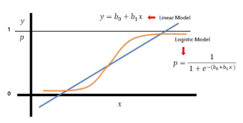
LogisticRegression

已知：
$$log\frac{p}{1-p}=\theta^Tx$$

$$Pp=P(y=1|x) ,即输入x预测为正样本的概率$$

求：
$$\theta$$

sklearn.linear_model.LogisticRegression(penalty=’l2’, dual=False, tol=0.0001, C=1.0, fit_intercept=True, intercept_scaling=1, class_weight=None, random_state=None, solver=’warn’, max_iter=100, multi_class=’warn’, verbose=0, warm_start=False, n_jobs=None, l1_ratio=None)

参数解释
1. penalty [defualt='l2']
- l2: l2 正则化
- l1,: l1 正则化
- elasticnet: elasticnet
- none:
2. dual [defualt=False]
- 对偶
- 'sag'求解器，默认值为1000
3. tol [defualt=0.0001]
- 误差项

C [defualt=1]
正则强度的倒数
fit_intercept [defualt=True]
是否添加截距（偏执）
add bias
intercept_scaling [defualt=1]
当使用 liner 解决方案的时候且 fit_intercept==True 时有效
solver [default=’liblinear’]
优化算法,可选项 liblinear, newton-cg, lbfgs, sag and saga
- lbfgs 因其有较好鲁棒性作为默认的求解方法
- saga 对于大数据集有更快的表现
- liblinear,坐标下降法，基于C++ LIBLINEAR使用，不适用多分类模型
- lbfgs”, “sag” and “newton-cg” 在高维数据上更快。
- sag solver uses Stochastic Average Gradient descent . 适用于较大数据集合，其求解速度快。
- saga solver 是 sag 的变体，唯一支持 penalty="elasticnet" 的求解器。
- lbfgs Broyden–Fletcher–Goldfarb–Shanno 算法（属于quasi-Newton methods），适合小数据集。
- 至于更大的数据集，推荐试试 sklearn.SGDClassifier 分类器使用 log-loss ，这样将更加快速。
- max_iter ： [defualt=100]
- 求解程序收敛所需的最大迭代次数
- multi_class:
- Setting multi_class to “multinomial” with these solvers learns a true multinomial

2. 基于支持向量机(SVM)的分类

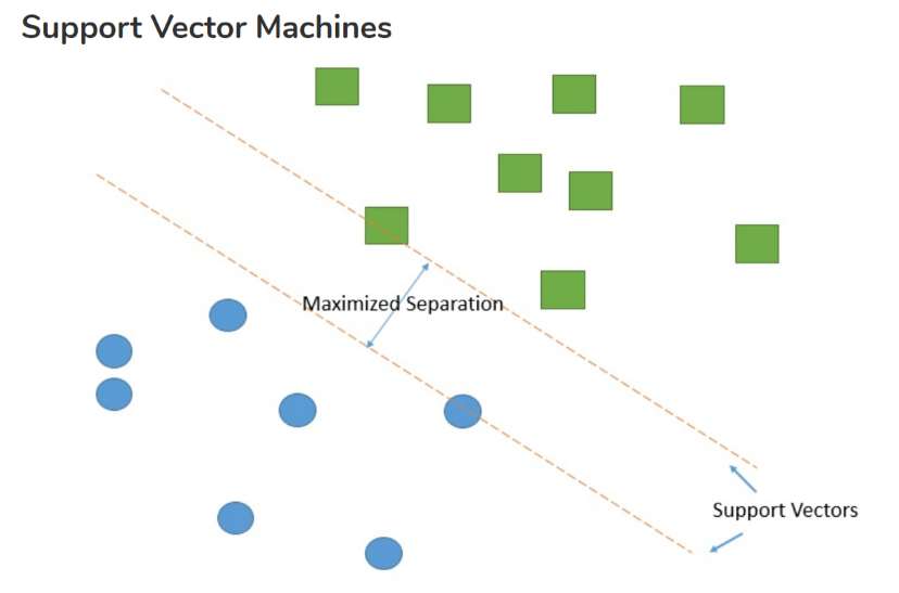
scikit-learn SVM算法库封装了libsvm（开源库：官方网站）和 liblinear的实现，仅仅重写了算法了接口部分。
其中支持向量机(SVM)对于分类问题有3个分类器：
1. SVC
2. NuSVC
3. LinearSVC

Note
- LIBSVM and LIBLINEAR are two popular open source machine learning libraries, both developed at the National Taiwan University and both written in C++ though with a C API

2.1. SVC

from sklearn.svm import SVC
scv=SVC(
    C=1.0,
    kernel='rbf',
    degree=3,
    gamma='auto_deprecated',
    coef0=0.0,
    shrinking=True,
    probability=False,
    tol=0.001,
    cache_size=200,
    class_weight=None,
    verbose=False,
    max_iter=-1,
    decision_function_shape='ovr',
    random_state=None,
)

参数说明
- C[defualt=1.0] 惩罚系数
SVM分类模型原型形式和对偶形式中的惩罚系数C，默认为1，一般需要通过交叉验证来选择一个合适的C。一般来说，如果噪音点较多时，C需要小一些。
- kernel[defualt="rbf"] 核函数
核函数有四种内置选择，不同核函数有不同的参数需要调整：
1. linear即线性核函数,
2. poly即多项式核函数,
3. rbf即高斯核函数,
4. sigmoid即sigmoid核函数

如果选择了这些核函数，对应的核函数参数在后面有单独的参数需要调。
- degree[defualt=3],ploy 核函数的深度
只对ploy核函数有效，对应d。
$$K(x,z)=(γ·x·z+r)dK(x,z)=(γ · x · z+r)d$$
- gamma[defualt='auto'=1/number−features]
poly多项式核函数中这个参数对应:γ,
$$K(x,z)=(γx∙z+r)dK(x,z)=(γx∙z+r)d$$
高斯核函数中这个参数对应γ:
$$K(x,z)=exp(γ||x−z||2)K(x,z)=exp(γ||x−z||2)$$
sigmoid核函数中这个参数对应γ
$$K(x,z)=tanh(γx∙z+r)K(x,z)=tanh(γx∙z+r)$$

默认为'`auto`',即=`1/number−features`

coef0[defualt=0]
多项式核函数中这个参数对应r
$$K(x,z)=(γx∙z+r)dK(x,z)=(γx∙z+r)d$$

sigmoid核函数中这个参数对应r
$$K(x,z)=tanh(γx∙z+r)K(x,z)=tanh(γx∙z+r)$$
class_weight[defualt="None"]样本权重
1. balanced，算法会自己计算权重，样本量少的类别所对应的样本权重会高。
2. None,如果你的样本类别分布没有明显的偏倚，则可以不管这个参数，选择默认的None
  指定样本各类别的的权重，主要是为了防止训练集某些类别的样本过多，导致训练的决策过于偏向这些类别。这里可以自己指定各个样本的权重，或者用balanced。
decision_function_shape[default='ovr'] 分类决策函数类型
1. 'ovo', 返回original
  one-vs-one ('ovo') decision function of libsvm which has shape
  (n_samples, n_classes * (n_classes - 1) / 2) 通常用于多分类问题，速度慢，一般用ovo
2. 'ovr', 返回一个one-vs-rest ('ovr') decision function of shape
  (n_samples, n_classes) as all other classifiers。相对简单，但分类效果相对略差，速度快。
  Whether to return a , or the . However, one-vs-one
  ('ovo') is always used as multi-class strategy.
cache_size[defualt=200] 缓存大小
LinearSVC计算量不大，因此不需要这个参数在大样本的时候，缓存大小会影响训练速度，因此如果机器内存大，推荐用500MB甚至1000MB。默认是200MB。

2.2. NuSVC

与SVC 一样，使用libsvm进行开发的
Similar to SVC but uses a parameter to control the number of support vectors.
控制支持向量的数量

from sklearn.svm import NuSVC

nusvc=NuSVC(
    cache_size=200, 
    class_weight=None, 
    coef0=0.0,
    decision_function_shape='ovr', degree=3, 
    gamma='auto_deprecated',
    kernel='rbf', 
    max_iter=-1, 
    nu=0.5, 
    probability=False, 
    random_state=None,
    shrinking=True, 
    tol=0.001, verbose=False)

参数说明
- nu An upper bound on the fraction of training errors and a lower bound of the fraction of support vectors. Should be in the interval (0, 1].

2.3. LinearSVC

LinearSVC 是线性分类，也就是不支持各种低维到高维的核函数，仅仅支持线性核函数，对线性不可分的数据不能使用。
- multi_class 分类决策
可以选择 ovr 或者 crammer_singer ovr和SVC和nuSVC中的decision_function_shape对应的ovr类似。'crammer_singer'是一种改良版的'ovr'，说是改良，但是没有比ovr好，一般在应用中都不建议使用。

3. 朴素贝叶斯

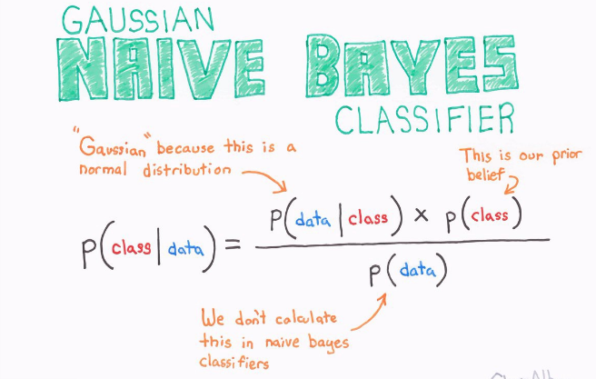
朴素贝叶斯是基于贝叶斯定理的一组有监督学习算法，即“简单”地假设每对特征之间相互独立。

另一方面，尽管朴素贝叶斯被认为是一种相当不错的分类器，但却不是好的估计器(estimator)，所以不能太过于重视从 predict_proba 输出的概率。

朴素贝叶斯一共有三种方法，分别是：
1. 高斯朴素贝叶斯
2. 多项式分布贝叶斯
3. 伯努利朴素贝叶斯

如果样本特征的分布大部分是连续值，使用高斯朴素贝叶斯GaussianNB会比较好。
如果如果样本特征的分大部分是多元离散值，使用多项式分布贝叶斯MultinomialNB比较合适。
如果样本特征是二元离散值或者很稀疏的多元离散值，应该使用伯努利朴素贝叶斯BernoulliNB。

3.1. 高斯朴素贝叶斯

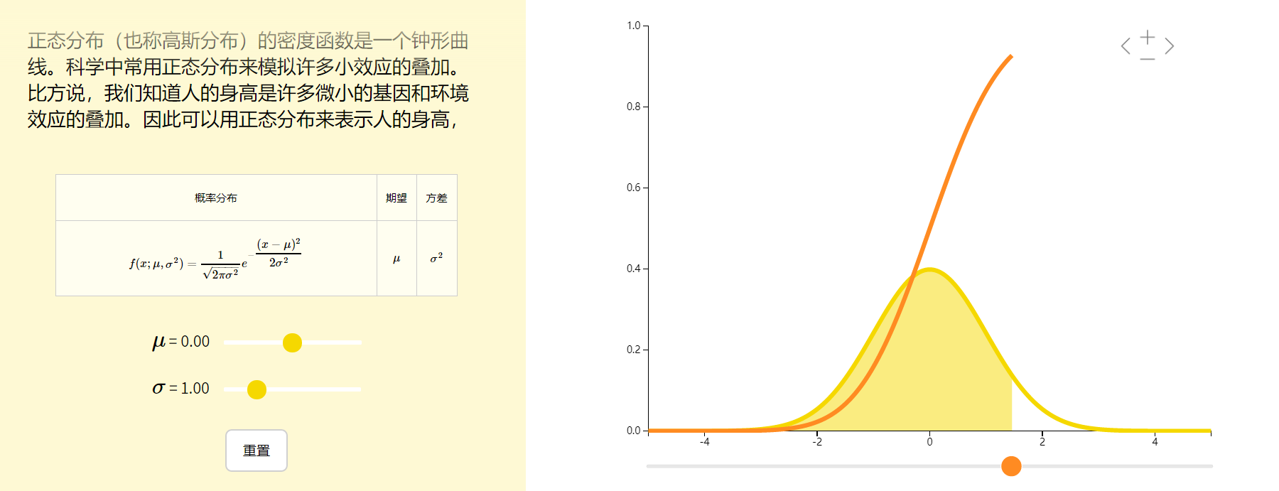
高斯朴素贝叶斯算法是假设特征的可能性(即概率)为高斯分布。
根据样本$D(x_i)$算出均值$\mu$和方差$\sigma$，再求得概率。
$$P(x_i|y)=\frac{1}{\sqrt{2\pi\sigma^2}}exp{(-\frac{x_i-\mu^2}{2\sigma^2})}$$
参数 $\sigma_y$ 和 $\mu_y$ 使用最大似然法估计。

from sklearn.naive_bayes import GaussianNB
gnb = GaussianNB(priors=None)

参数说明
priors:先验概率大小，如果没有给定，模型则根据样本数据自己计算（利用极大似然法）。

3.2. 伯努利朴素贝叶斯

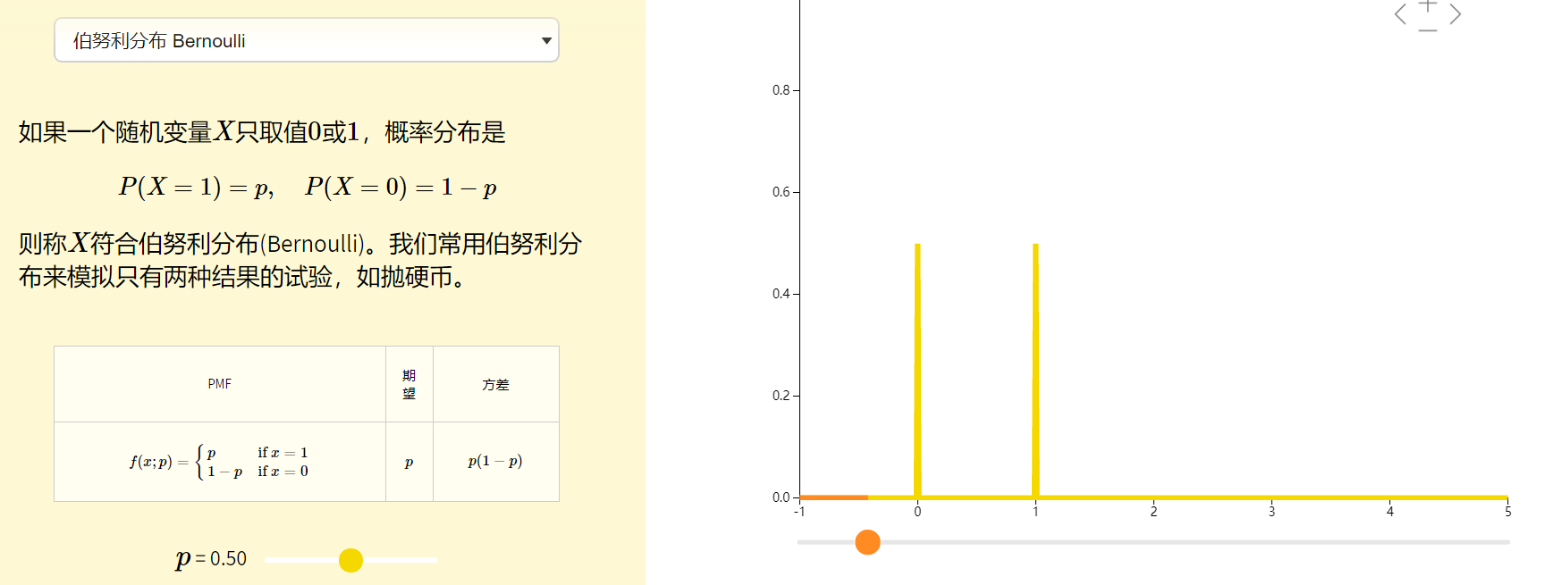
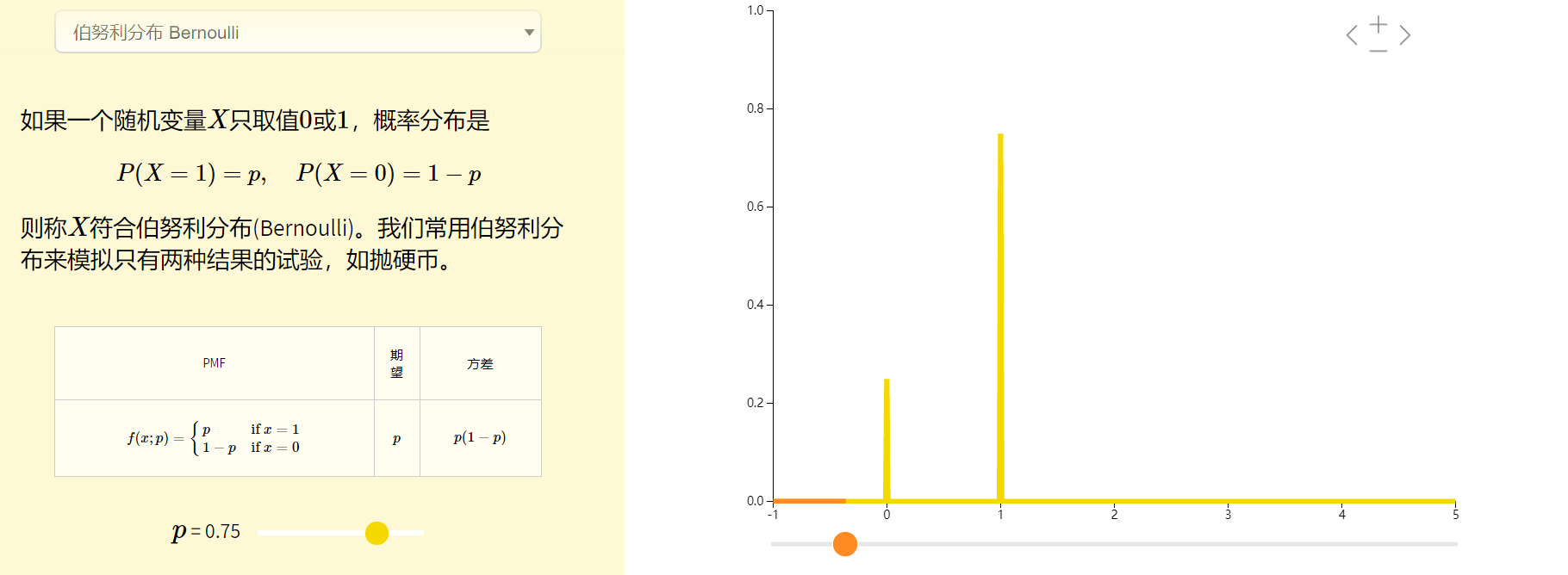
class sklearn.naive_bayes.BernoulliNB(alpha=1.0, binarize=0.0, fit_prior=True, class_prior=None)

参数说明
alpha:平滑因子，与多项式中的alpha一致。

binarize:样本特征二值化的阈值，默认是0。如果不输入，则模型会认为所有特征都已经是二值化形式了；如果输入具体的值，则模型会把大于该值的部分归为一类，小于的归为另一类。

fit_prior:是否去学习类的先验概率，默认是True

class_prior:各个类别的先验概率，如果没有指定，则模型会根据数据自动学习，每个类别的先验概率相同，等于类标记总个数N分之一。

3.3. 多项式分布贝叶斯

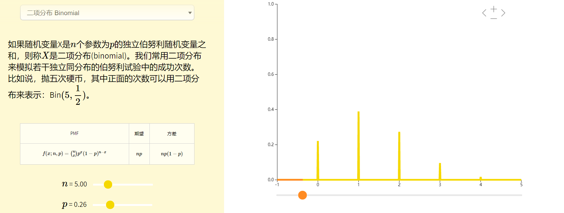
多项式分布（Multinomial Distribution）是二项式分布的推广，二项分布是随机结果值只有两个(投硬币的结果-正反面--2种)，多项式分布是指随机结果值有多个(摇骰子的结果-6种)。

# 多项分布朴素贝叶斯
from sklearn import datasets
iris = datasets.load_iris()

from sklearn.naive_bayes import MultinomialNB
clf = MultinomialNB()
clf = clf.fit(iris.data, iris.target)
y_pred=clf.predict(iris.data)
print("多项分布朴素贝叶斯，样本总数： %d 错误样本数 : %d" % (iris.data.shape[0],(iris.target != y_pred).sum()))

4. k近邻分类器（knn）

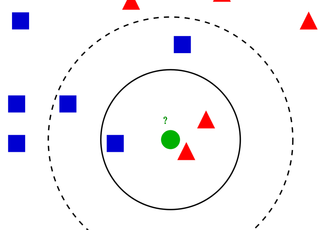
from sklearn.neighbors import KNeighborsClassifier

KNeighborsClassifier(n_neighbors=5, weights='uniform', algorithm='auto', leaf_size=30, p=2, metric='minkowski', metric_params=None, n_jobs=None, **kwargs)

参数解释
- n_neighbors:k 近邻的k
- weights: 权重
- algorithm: 如何找到最近的k个邻居--计算的算法，可选项为 ‘auto’, ‘ball_tree’, ‘kd_tree’, ‘brute’

- `ball_tree`: 构建 BallTree
  - 通过这种方法构建的树要比 KD 树消耗更多的时间, 但是这种数据结构对于高结构化的数据是非常有效的, 即使在高维度上也是一样.
- `kd_tree`:构建 KD树。
  - 虽然 KD 树的方法对于低维度 (D < 20) 近邻搜索非常快, 当 D 增长到很大时, 效率变低: 这就是所谓的 “维度灾难” 的一种体现。
- `brute`: 暴力搜索
- `auto` will attempt to decide the most appropriate algorithm based on the values passed to fit method.

leaf_sizeint, optional (default = 30) 争对KD树和BallTree 树
metric string or callable, default ‘minkowski’ 明科夫斯基距离
pinteger, optional (default = 2) p值，明科夫斯基距离的平方
n_jobs[Defualt=None]:计算使用的线程数量None means 1 ,-1 ==core of cups

5. 决策树分类

5.1. 单一决策树分类器

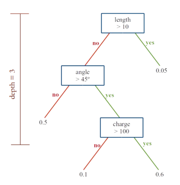
Decision Tree Classifiers/Random Forests

sklearn.tree.DecisionTreeClassifier(criterion='gini', splitter='best', max_depth=None, min_samples_split=2, min_samples_leaf=1, min_weight_fraction_leaf=0.0, max_features=None, random_state=None, max_leaf_nodes=None, min_impurity_decrease=0.0, min_impurity_split=None, class_weight=None, presort='deprecated', ccp_alpha=0.0)

参数说明

criterion:{“gini”, “entropy”}, default=”gini”

splitter, default=”best”

5.2. 随机森林分类器

sklearn.ensemble.RandomForestClassifier(n_estimators=100, criterion='gini', max_depth=None, min_samples_split=2, min_samples_leaf=1, min_weight_fraction_leaf=0.0, max_features='auto', max_leaf_nodes=None, min_impurity_decrease=0.0, min_impurity_split=None, bootstrap=True, oob_score=False, n_jobs=None, random_state=None, verbose=0, warm_start=False, class_weight=None, ccp_alpha=0.0, max_samples=None)

参数说明
n_estimators=100,
criterion='gini'

参考资料：官方文档

6. 线性判别分析 LDA

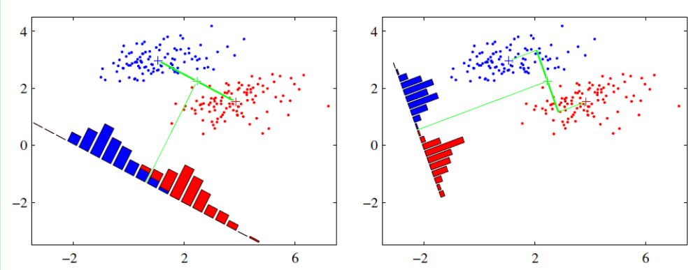
最大类间间距，最小类内间距

sklearn.discriminant_analysis.LinearDiscriminantAnalysis(solver='svd', shrinkage=None, priors=None, n_components=None, store_covariance=False, tol=0.0001)[source]

参数说明

solver
- 默认solver为svd。

svd 奇异值分解，它既能进行分类又能进行降维，不依赖于协方差矩阵的计算。在功能数量众多的情况下，这可能是一个优势。但是，“svd” solver不能用于shrinkage 。
lsqr 最小二乘法 solver 是一种有效的算法，只适用于分类。它支持shrinkage ，支持特征缩放（L2/L1 正则化）
eigen 特征值分解，它可以被用于 classification （分类）以及 transform （转换），可以用fit_transform()方法，可以降维。solver需要计算协方差矩阵，因此它可能不适合具有大量特征的, 支持特征缩放（L2/L1 正则化）

Kmean

from sklearn.cluster import KMeans


KMeans(n_clusters=8, init='k-means++', n_init=10, max_iter=300, tol=0.0001, precompute_distances='auto', verbose=0, random_state=None, copy_x=True, n_jobs=None, algorithm='auto')

参数说明

n_clusters : int
- 选取的n个簇

init : {'k-means++', 'random' or an ndarray}
- 簇位置的初始化方法
- 如果是np.array ,shape= (n_clusters, n_features)

n_init : int, default: 10
- 用不同的聚类中心初始化值运行算法的次数，最终解是在inertia(每个簇内到其质心的距离相加) 意义下选出的最优结果

max_iter : int, default: 300
- 最大迭代次数

tol : float, default: 1e-4
Relative tolerance with regards to inertia to declare convergence

precompute_distances : {'auto', True, False}
-　预计算距离，计算速度更快但占用更多内存。
　　1. auto：如果样本数乘以聚类数(n_samples*n_clusters)大于 12 million 的话则不预计算距离。
　　2. True：总是预先计算距离。
　　3. False：永远不预先计算距离。

verbose : int, default 0
Verbosity mode.是否输出详细信息，0 不输出

random_state : int, RandomState instance or None (default)
Determines random number generation for centroid initialization. Use
an int to make the randomness deterministic.
See :term:Glossary <random_state>.

copy_x : boolean, optional
When pre-computing distances it is more numerically accurate to center
the data first. If copy_x is True (default), then the original data is
not modified, ensuring X is C-contiguous. If False, the original data
is modified, and put back before the function returns, but small
numerical differences may be introduced by subtracting and then adding
the data mean, in this case it will also not ensure that data is
C-contiguous which may cause a significant slowdown.

n_jobs : int or None, optional (default=None)
- 计算使用的cpu数量
- 默认None=1，-1 表示最大

algorithm : "auto", "full" or "elkan", default="auto"
- 使用的算法
- full 是经典的EM 算法
- elkan elkan 算法利用了两边之和大于等于第三边,以及两边之差小于第三边的三角形性质，来减少距离的计算。
- "auto" 对稀疏矩阵使用elkan 算法，对稠密矩阵使用EM 算法

7. 参考资料

What are the differences between SVC, NuSVC, and LinearSVC?